Creating an auto-layout algorithm for graphs

In the last few months I worked on a finite state machine editor build on React Flow. At a certain point I wanted to import a configuration, that magically visualizes the state machine. I was in the need of a graph layout algorithm. A few years back, I have implemented a similar feature for a workflow editor. The biggest problem to solve? Ensuring the resulting visualization is understandable and readable. This requires a solid algorithm.

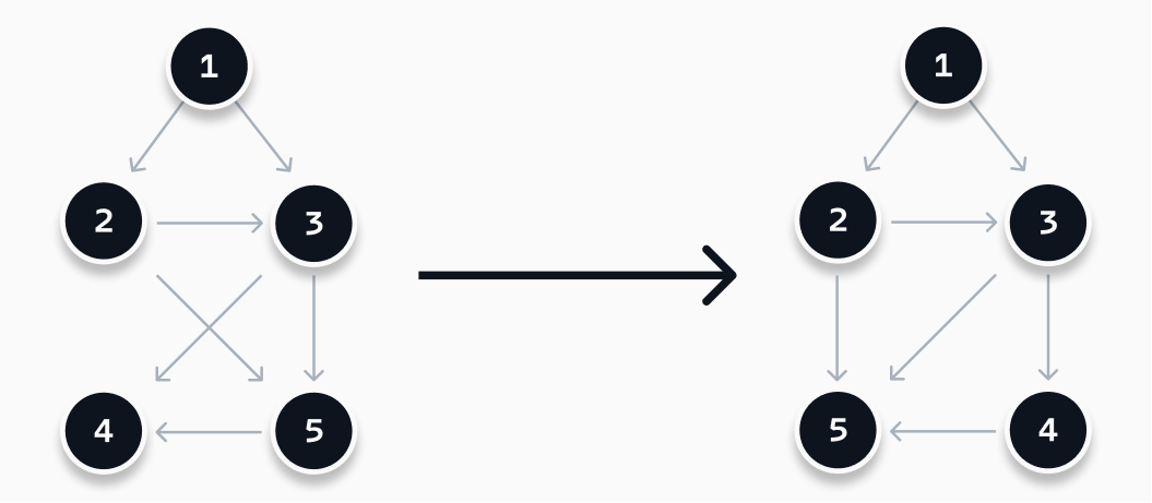
If all nodes in the graph are scattered across the screen, it will become hard to follow the lines between them. The approach I took is based on the paper "A technique for drawing directed graphs (1993)". It is a technique based on finding a (local) minimum in the number of crossing edges, as visualized below. My implementation consists out of three steps: (1) rank all nodes, (2) optimize the order of the nodes, and (3) determine the position of each node.

Rank all nodes #

The first step of the algorithm is to rank all nodes. All graphs have an initial node. It is the starting point of a process/workflow or the initial state of a state machine. This particular node is placed in rank 0. With this starting point, we follow three steps to determine an initial rank for all the nodes.

1. Determine the initial rank of each node. The rank of a node equals the length of the shortest route between this node and the initial node. The rank can be determined using a breadth-first search algorithm.
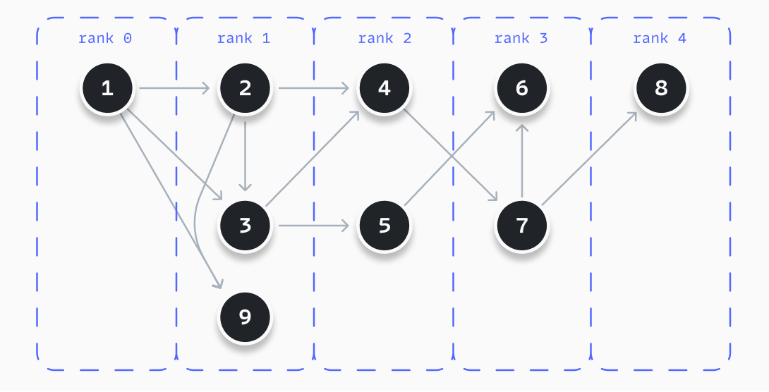
2. Determine all possible paths from the starting node, using a depth-first search algorithm, like displayed below.
3. Order all nodes within a rank, based on their occurrence in the longest path. Nodes in longer paths are placed higher within a rank.

function getPaths(nodeId, edges, path = [], paths = []) {
  const children = edges.filter((e) => e.source === nodeId);

  const _path = [...path, nodeId];

  // To avoid cycles in paths
  if (path.includes(nodeId)) {
    paths.push(path);
  } else if (!children || children.length === 0) {
    paths.push(_path);
  } else {
    children.map((c) => getAllPaths(c.target, edges, _path, paths));
  }

  return paths.sort();
}

The example below visualizes a result when following these steps. You can see that all nodes are ranked as described. In this example, node 4 is placed at the top of rank 2, as it appears in the longest path, while node 5 does not.

Optimize the order of the nodes #

The above visualization shows that ranking nodes following these steps can produce readable results. But, improvements can be achieved. As this is a so-called 'NP-hard' problem, there is no perfect solution possible. But, by following a certain sequence of steps, several times until we hit a boundary condition, we can approach a (local) optimum. Or you know, the minimum number of crossing edges. This is called a heuristic.

A vital part of this heuristic is the ability to give a configuration a score. This score is used to compare various mutations of the graph and find a (local) best based on this score. As mentioned before, the idea of this algorithm revolves around minimizing the amount of crossing edges. Thus, our score needs to be related to that. An easy scoring mechanism can be:

• Count the number of edges that have the source and target in the same rank and are not next to each other. You can also count the number of nodes between them. This would give a higher score when the source and target are further apart.
• Look at all combinations of ranks and count all edges between these two ranks (regardless of their directions), where the condition shown below is met.

// Assumes both edges have the source in a lower rank
// edge = [sourceIndexInRank, targetIndexInRank]

function edgesCross(edge1, edge2) {
  if (edge1[0] < edge2[0] && edge1[1] > edge2[1]) {
    return true;
  } else if (edge1[0] < edge2[0] && edge1[1] > edge2[1]) {
    return true;
  }
  return false;
}

With the scoring mechanism determined, it's time to look at the actual heuristic. The heuristic I choose is iteratively moving through all ranks and swaps two adjacent nodes. If they improve (or at least not worsen) the score, the mutation stays, for now. As this mechanism is not perfect, as not all possible mutations are explored, we can apply this heuristic for a maximum of X times, to balance between performance and optimal results. The detailed steps of the heuristic are outlined below.

1. Let i = 1 and move to rank[i].
2. Let j = 0. Swap rank[i][j] with rank[i][j + 1].
3. Determine the score of the new graph, if the score becomes worse, reverse the mutation, else keep the mutation.
4. Set j = j + 1 if possible, else set i = i + 1 if possible, and repeat step 2. If neither is possible, proceed to step 5.
5. If the resulting graph has a better score, repeat step 1 for the new graph, for a maximum of X times. Else you found a (local) optimum.

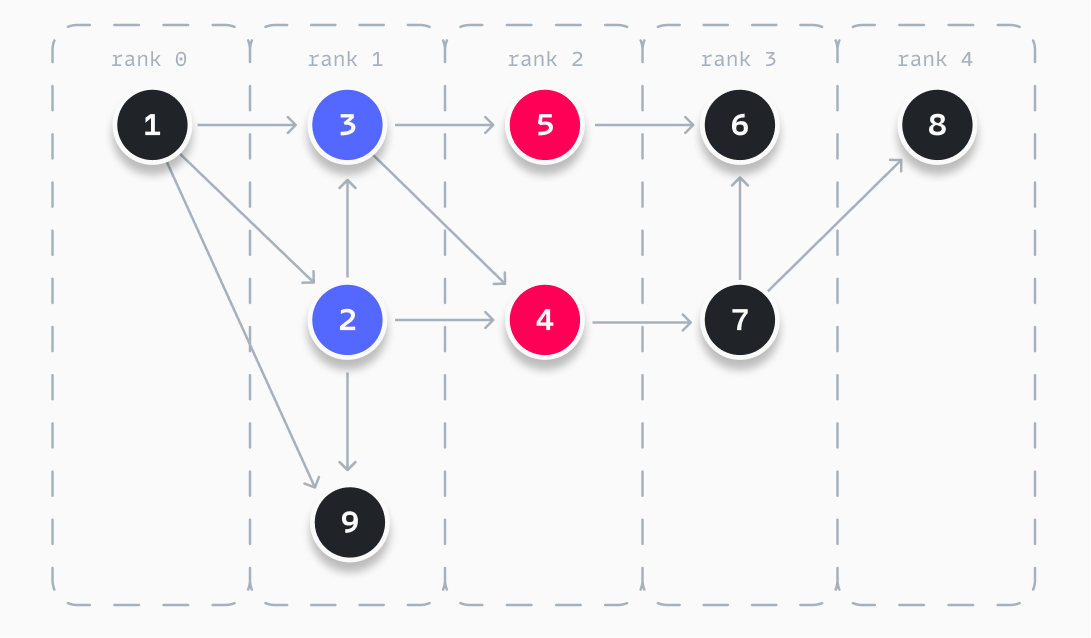
The example graph used before has two crossing edges. By applying the above heuristic, we can optimize this by applying two mutations, as visualized above. When we swap nodes 2 and 3, we are getting the same score of 2. This means to apply the mutation and continue. Nodes 2 and 9 cannot be swapped, as it worsens the score of the graph. When swapping 4 and 5 after swapping 2 and 3, we find a perfect score and thus our resulting graph.

Determine the position of each node #

After we have optimized all our ranks of nodes, it is time to determine the position of each node. Various routes can be taken, but the easiest is to place nodes in a grid. In the end, our ranks are a grid. This is illustrated below, using the running example from the previous sections. By using a grid, you create several options for yourself to lay out your graph. You can take a traditional route, like the visualization shown in the previous section.

You could also go for a more balanced graph, where all nodes are laid out around a centerline. In your initial rank, you always have one node. Depending on the orientation of your graph, this initial node is placed on a horizontal or vertical centerline. As you can see in the example, nodes 1, 2, and 8 all line on this centerline, instead of having five nodes on a single line.

|   |   | 3 |   |   |   |   |   |   |
|   |   |   |   | 5 |   | 6 |   |   |
| 1 |   | 2 |   |   |   |   |   | 8 |
|   |   |   |   | 4 |   | 7 |   |   |
|   |   | 9 |   |   |   |   |   |   |

Wrapping up #

Solving the automatic (or magical) layout of a directed graph (or state machine) is one of the most fun challenges I ever had. By doing research I found an algorithm I understood and could put in place. The described algorithm proves to be effective for small to medium-sized graphs. Most of these graphs are not spiderwebs and have limited edges (e.g. 2-3 outgoing edges per node). Don't believe me? I use the algorithm in an online state machine editor I have created. But, it is a heuristic and by definition not perfect. Some improvements I can think of already are:

• Make it possible to change the weight of certain types of crossing edges (e.g. edges crossing with a rank have a higher weight). This allows you to control the algorithm to your own needs.
• Allow for nodes to move between ranks during the optimization step. This is a helpful improvement when you have a graph with a fixed start and end node, but a big variation in the length of paths.
• Optimize how mutations and which mutations are applied. Check only adjacent ranks to improve the performance for example. This can worsen the result though.